Image classification is a challenging task for computers. Convolutional neural networks represent one data-driven approach to this challenge. This post will be about image representation and the layers that make up a convolutional neural network.

---

Neural Network Structure

This post is the second in a series about understanding how neural networks learn to separate and classify visual data. In the last post, I went over why neural networks work: they rely on the fact that most data can be represented by a smaller, simpler set of features. Neural networks are made of many nodes that learn how to best separate training data into classes or other specified groups, and many layers of nodes can create more and more complex boundaries for separating and grouping this data.

---

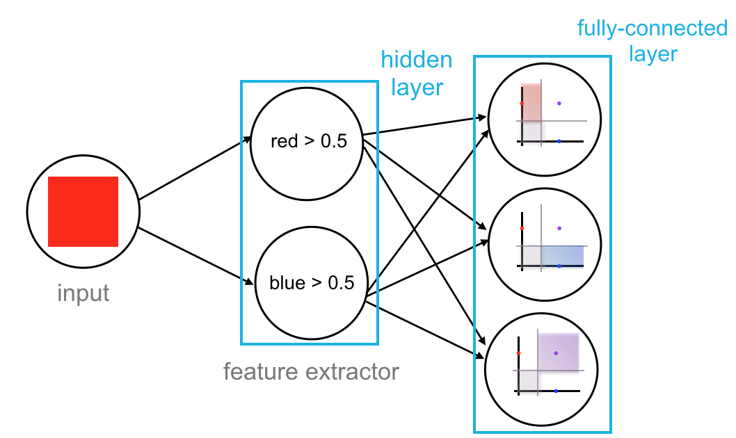
Image Classification

In the case of image classification, we want a neural network that looks at an image and outputs the correct class for that image. Let’s take an image of a car as an example.

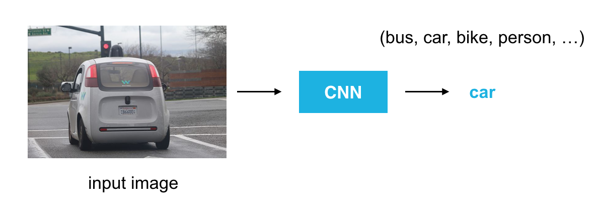
It’s simple for us to look at this image and identify the car, but when we give a neural network this image, what does it see?

Images as Grids of Pixels

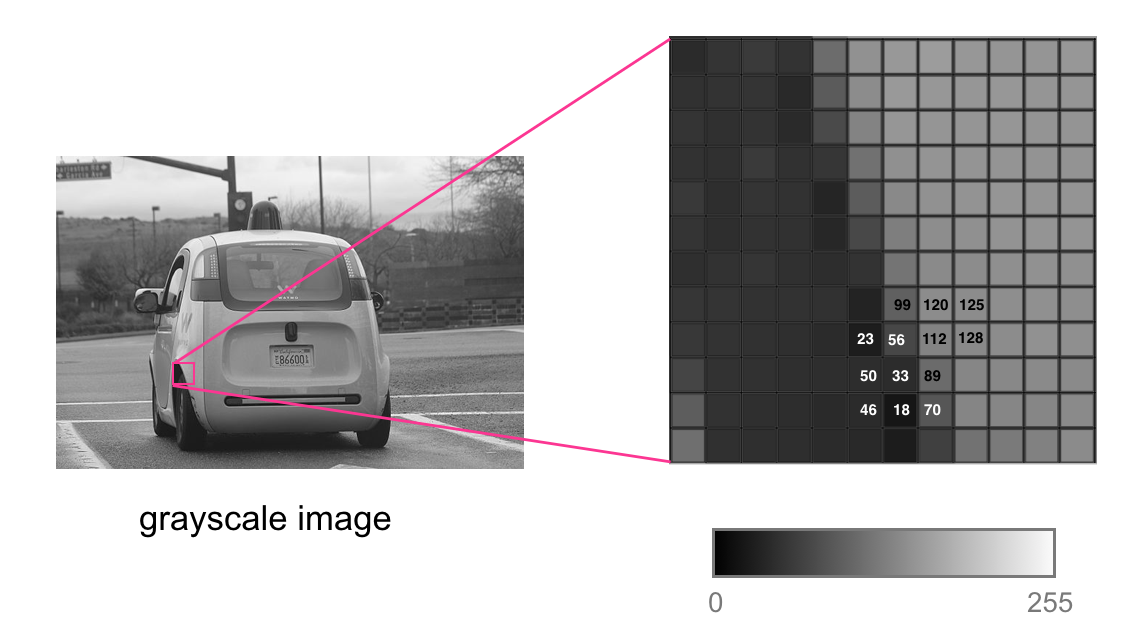
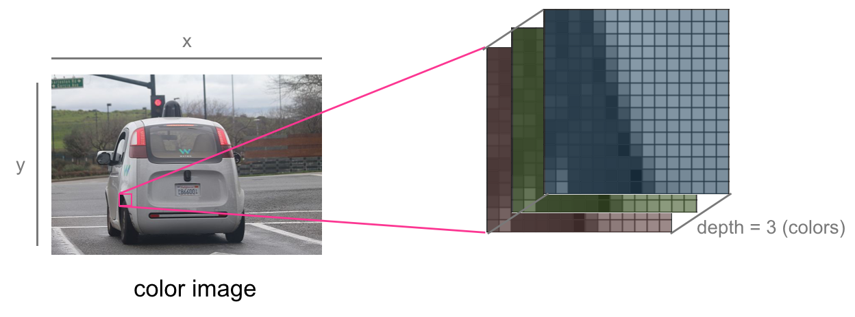
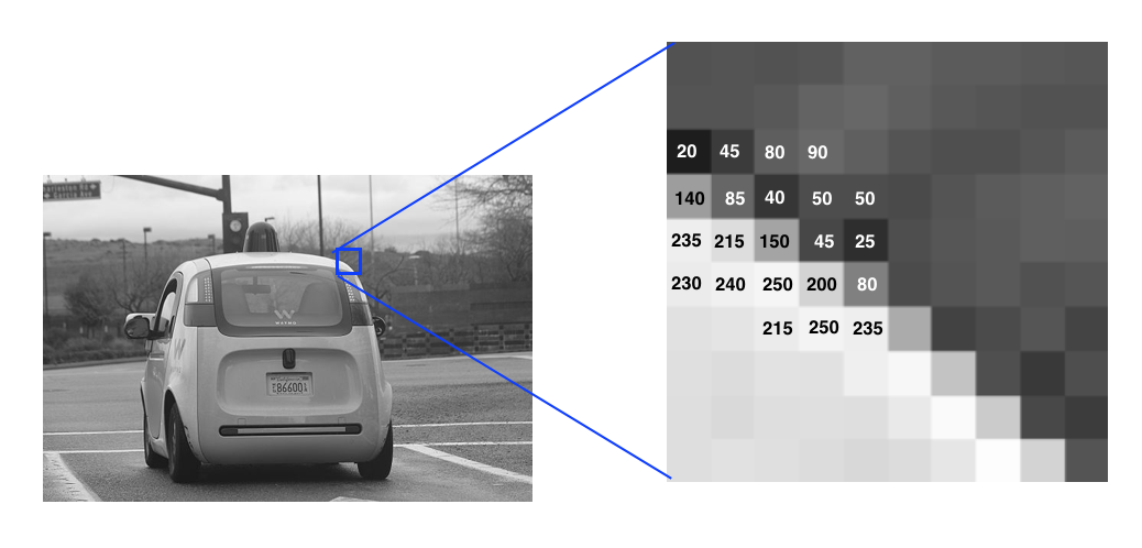
An image is seen by a neural network (and by computers) as a grid of numerical values. Below, you’ll see a zoomed-in portion of a grayscale image of a car. The image is broken up into a fine grid, and each of the grid cells is called a pixel. For grayscale images, each pixel has a value between 0 and 255, where 0 is black and 255 is white; shades of gray are anywhere in between.

For a standard color image, there are red, green, and blue pixel values for each (x,y) pixel location. We can think of this as a stack of three images, one for each of the red, green, and blue color components. You may see a color pixel value written as a list of three numerical values. For example, for an RGB pixel value, [255,0,0] is pure red and [200,0,200] is purple. In this way, we can think of any image as a 3D volume with some width, height, and color depth. Grayscale images have a color depth of 1.

To create an image classifier, we need an algorithm that can look at these pixel values and classify this image as a car. We also want a classifier to be able to detect this car under varying light conditions (at night or during a sunny day), and we want the classifier to generalize well so that it can recognize a variety of cars in different environments and in different poses.

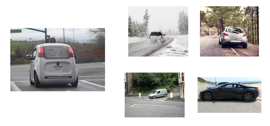
If you look at just a small sample of car images, you can see that the pixel values are really different for each of these images. So, the challenge becomes: how can we create a classifier that, for any of these grids of pixel values, will be able to classify each one of them as a car.

Data-Driven Approach

Since there is no clear way to create a set of rules about pixel values that make up a car, we’ll instead take a data-driven approach:

1. Collect a set of images with true class labels.
2. Train a model to produce an accurate, predicted class label.

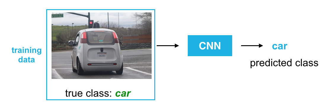
In this example, we’ll plan to train a convolutional neural network. As this network trains, it should learn what parts of a car are important to recognize, such as wheels and windows, and it should be general enough to recognize cars in a variety of positions and environments.

---

Convolutional Neural Network

To approach this image classification task, we’ll use a convolutional neural network (CNN), a special kind of neural network that can find and represent patterns in 3D image space. Many neural networks look at individual inputs (in this case, individual pixel values), but convolutional neural networks can look at groups of pixels in an area of an image and learn to find spatial patterns.

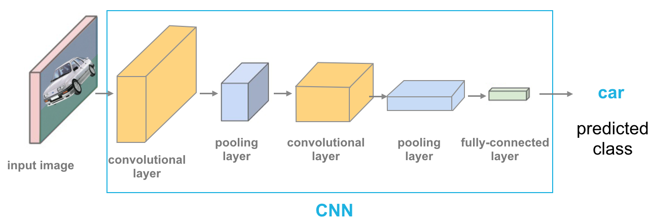
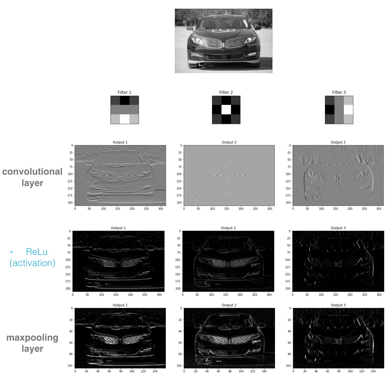
Every CNN is made up of multiple layers, the three main types of layers are convolutional, pooling, and fully-connected, as pictured below. Typically, you’ll see CNN’s made of many layers, especially convolutional and pooling layers. Each of these layers is made of nodes that look at some input data and produce an output, so let’s go over what each of these layers does!

Convolutional Layer

The convolutional layer can be thought of as the feature extractor of this network, it learns to find spatial features in an input image. This layer is produced by applying a series of many different image filters, also known as convolutional kernels, to an input image. These filters are very small grids of values that slide over an image, pixel-by-pixel, and produce a filtered output image that will be about the same size as the input image. Multiple kernels will produce multiple filtered, output images.

Say we have four different convolutional kernels, these will produce four different, filtered images as output. The idea is that each filter will extract a different feature from an input image and these features will eventually help to classify that image, for example, one filter might detect the edges of objects in that image and another might detect unique patterns in color. These filters, stacked together, are what make up a convolutional layer.

---

High-pass Filter

Let’s take a closer look at one type of convolutional kernel: a high-pass image filter. High-pass filters are meant to detect abrupt changes in intensity over a small area. So, in a small patch of pixels, a high-pass filter will highlight areas that change from dark to light pixels (and vice versa). I’ll be looking at patterns of intensity and pixel values in a grayscale image.

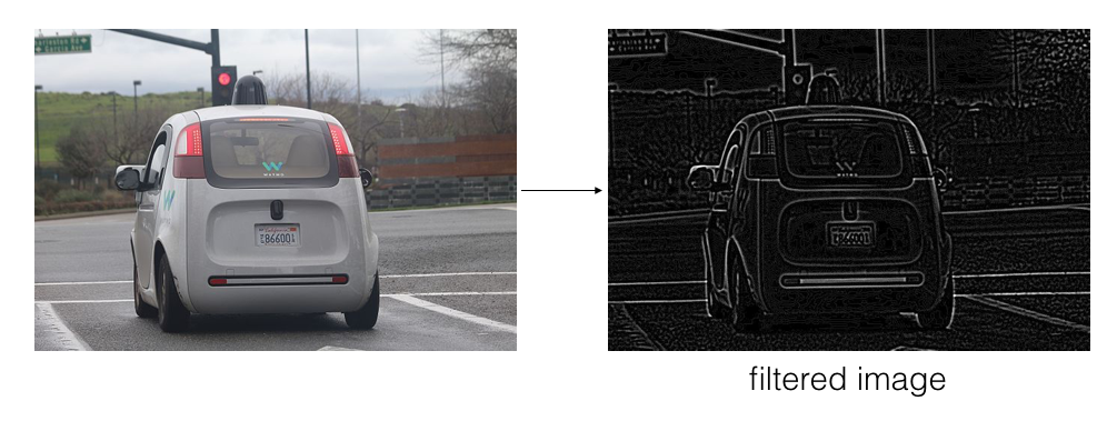
For example, if we put an image of a car through a high-pass filter, we expect the edges of the car, where the pixel values change abruptly from light to dark, to be detected. The edges of objects are often areas of abrupt intensity change and, for this reason, high-pass filters are sometimes called “edge detection filters.”

Convolutional Kernels

The filters I’ll be talking about are in the form of matrices, also called convolutional kernels, which are just grids of numbers that modify an image. Below is an example of a high-pass filter, a 3x3 kernel that does edge detection.

You may notice that all the elements in this 3x3 grid sum to zero. For an edge detection filter, it’s important that all of it’s’ elements sum to zero because it’s computing the difference or change between neighboring pixels. If these pixel weights did not add up to zero, then the calculated difference would be either positively or negatively weighted, which has the effect of brightening or darkening the entire filtered image, respectively.

Convolution

To apply this filter to an image, an input image, F(x,y), is convolved with the kernel, K. Convolution is represented by an asterisk (not to be mistaken for multiplication). It involves taking a kernel, which is our small grid of numbers, and passing it over an image, pixel-by-pixel, creating another edge-detected output image whose appearance depends on the kernel values.

I’ll walk through a specific example, using the 3x3 edge detection filter. To better see the pixel-level operations, I’ll zoom in on the image of the car.

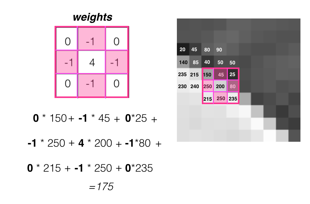
For every pixel in this grayscale image, we place our kernel over it, so that the selected pixel is at the center of the kernel, and perform convolution. In the below image, I’m selecting a center pixel with a value of 200, as an example.

The steps for a complete convolution are as follows:

1. Multiply the values in the kernel with their matching pixel value. So, the value in the top left of the 3x3 kernel (0), will be multiplied by the pixel value in that same corner in our image area (150).
2. Sum all these multiplied pairs of values to get a new value, in this case, 175. This value will be the new pixel value in the filtered output image, at the same (x,y) location as the selected center pixel.

This process repeats for every pixel in the input image, until we are left with a complete, filtered output.

Weights

Before we move on, I want to add a bit of terminology. The values inside a kernel, which are multiplied by their corresponding pixel value, are called weights. This is because they determine how important (or how weighty) a pixel is in forming a new, output image. You’ll notice that the center pixel has a weight of 4, which means it is heavily, positively weighted. Out of all the pixels in a 3x3 patch, the center pixel will be the most important in determining the value of the pixel in the output, filtered image.

The kernel also contains negative weights with a value of -1. These correspond to the pixels that are directly above and below, and to the left and right, of the center pixel. These pixels are closest to the center pixel and, because they are symmetrically distributed around the center, we can say that this kernel will detect any change in intensity around a center pixel on its left and right sides and on its top and bottom sides.

Image Borders

The only pixels for which convolution doesn’t work are the pixels at the borders of an image. A 3x3 kernel cannot be perfectly placed over a center pixel at the edges or corners of an image. In practice, there are a few ways of dealing with this, the most common ways are to either pad this image with a border of 0’s (or another grayscale value) so that we can perfectly overlay a kernel on all the pixel values in the original image, or to ignore the pixel values at the borders of the image, and only look at pixels where we can completely overlay the 3x3 convolutional kernel.

Often, there is not a lot of useful information at the border of an image, but if you do choose to ignore this information, every filtered image will be just a little bit smaller than the original input image. For a 3x3 kernel, we’ll actually lose a pixel from each side of an image, resulting in a filtered output that is two pixels smaller in width and in height than the original image. You can also choose to make larger filters. 3x3 is one of the smallest sizes and it’s good for looking at small pixel areas, but if you are analyzing larger images you may want to increase the area and use kernels that are 5x5, 7x7, or larger. Usually, you want an odd number so that the kernel nicely overlays a center pixel.

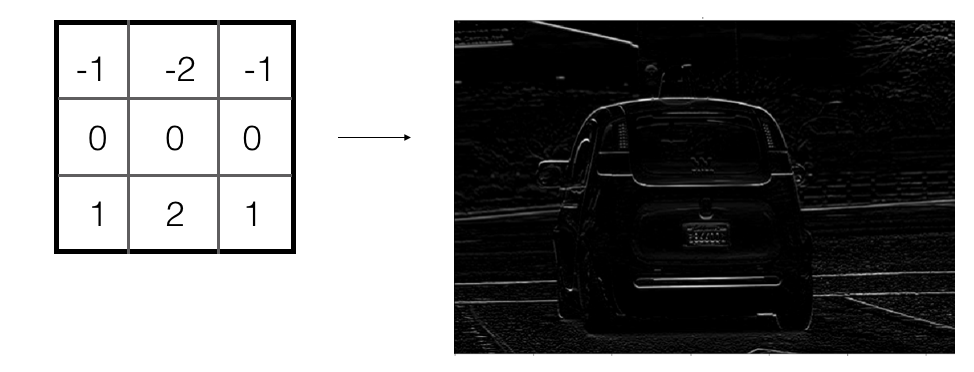
Above is another type of edge detection filter; this filter is computing the difference around a center pixel but it’s only looking at the bottom row and top row of surrounding pixel values. The result is a horizontal edge detector. In this way, you can create oriented edge detectors!

So, these convolutional kernels, when applied to an image, make a filtered image and several filtered images make a convolutional layer.

---

Activation Function

Recall that grayscale images have pixels values that fall in a range from 0-255. However, neural networks work best with scaled “strength” values between 0 and 1 (we briefly mentioned this in the last post). So, in practice, the input image to a CNN is a grayscale image with pixel values between 0 (black) and 1 (white); a light gray may be a value like 0.78. Converting an image from a pixel value range of 0-255 to a range of 0-1 is called normalization. Then, this normalized input image is filtered and a convolutional layer is created. Every pixel value in a filtered image, created by a convolution operation, will fall in a different range; there may even be pixel values that are negative.

To account for this change in pixel value, following a convolutional layer, a CNN applies an activation function that transforms each pixel value.

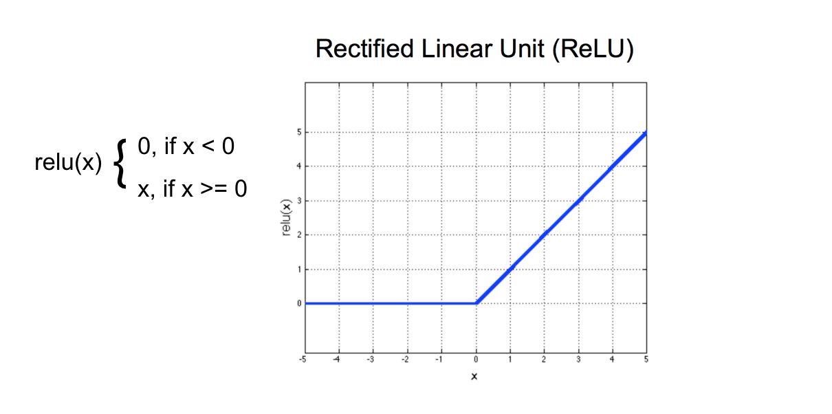
In a CNN, you’ll often use a ReLu (Rectified Linear Unit) activation function; this function simply turns all negative pixel values into 0’s (black). For an input, x, the ReLU function returns x for all values of x > 0, and returns 0 for all values of x ≤ 0. An activation function also introduces nonlinearity into a model, and this means that the CNN will be able to find nonlinear thresholds/boundaries that effectively separate and classify some training data.

---

Maxpooling Layer

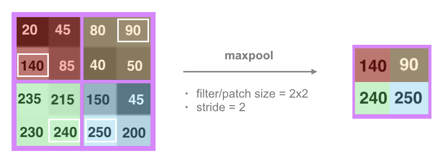
After a convolutional layer comes a pooling layer; the most common type of pooling layer is a maxpooling layer. Each of these layers looks at the pixel values in an image, so, to describe maxpooling, I’ll focus on a small pixel area. First, a maxpooling operation breaks an image into smaller patches, often 2x2 pixel areas.

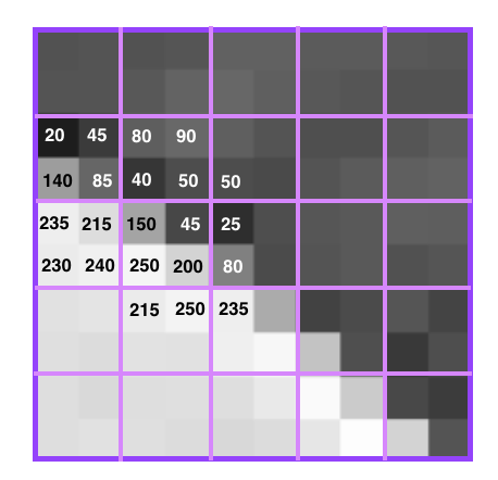
Let’s zoom in even further on four of these patches. A maxpooling layer is defined by the patch size, 2x2, and a stride. The patch can be thought of as a 2x2 window that the maxpooling layer looks at to select a maximum pixel value. It then moves this window by some stride across and down the image. For a patch of size 2x2 and a stride of 2, this window will perfectly cover the image. A smaller stride would see some overlap in patches and a larger stride would miss some pixels entirely. So, we usually see a patch size and a stride size that are the same.

For each 2x2 patch, a maxpooling layer looks at each value in a patch and selects only the maximum value. In the red patch, it selects 140, in the yellow, 90, and so on, until we are left with four values from the four patches.

Now, you might be wondering why we would use a maxpooling layer in the first place, especially since this layer is discarding pixel information. We use a maxpooling layer for a few reasons.

First, dimensionality reduction; as an input image moves forward through a CNN, we are taking a fairly flat image in x-y space and expanding its depth dimension while decreasing its height and width. The network distills information about the content of an image and squishes it into a representation that will make up a reasonable number of inputs that can be seen by a fully-connected layer. Second, maxpooling makes a network resistant to small pixel value changes in an input image. Imagine that some of the pixel values in a small patch are a little bit brighter or darker or that an object has moved to the right by a few pixels. For similar images, even if a patch has some slightly different pixel values, the maximum values extracted in successive pooling layers, should be similar. Third, by reducing the width and height of image data as it moves forward through the CNN, the maxpooling layer mimics an increase in the field of view for later layers. For example, a 3x3 kernel placed over an original input image will see a 3x3 pixel area at once, but that same kernel, applied to a pooled version of the original input image (ex. an image reduced in width and height by a factor of 2), will see the same number of pixels, but the 3x3 area corresponds to a 2x larger area in the original input image. This allows later convolutional layers to detect features in a larger region of the input image.

There are also other kinds of networks that do not use maxpooling, such as Capsule Networks, which you can read about in a separate blog post.

---

Fully-connected Layer

At the end of a convolutional neural network, is a fully-connected layer (sometimes more than one). Fully-connected means that every output that’s produced at the end of the last pooling layer is an input to each node in this fully-connected layer. For example, for a final pooling layer that produces a stack of outputs that are 20 pixels in height and width and 10 pixels in depth (the number of filtered images), the fully-connected layer will see 20x20x10 = 4000 inputs. The role of the last fully-connected layer is to produce a list of class scores, which you saw in the last post, and perform classification based on image features that have been extracted by the earlier convolutional and pooling layers; so, the last fully-connected layer will have as many nodes as there are classes.

---

CNN Layers, Summary

CNN’s are made of a number of layers: a series of convolutional layers + activation and maxpooling layers, and at least one, final fully-connected layer that can produce a set of class scores for a given image. The convolutional layers of a CNN act as feature extractors; they extract shape and color patterns from the pixel values of training images. It’s important to note that the behavior of the convolutional layers, and the features they learn to extract, are defined entirely by the weights that make up the convolutional kernels in the network. A CNN learns to find the best weights during training using a process called backpropagation, which looks at any classification errors that a CNN makes during training, finds which weights in that CNN are responsible for that error, and changes those weights accordingly.

---

PyTorch Code Examples

If you’d like to see how to create these kinds of CNN layers using PyTorch, take a look at my Github, tutorial repository. You may choose to skim the code and look at the output or set up a local environment and run the code on your own computer (instructions for setting up a local environment are documented in the repository readme).

Convolutional layers, activation functions, and maxpooling layers are in the first notebook: 1. Convolutional NN Layers, Visualization.

Note that, in the first notebook, I’ve explicitly defined the weights of the convolutional layer. However, when we get to training a neural network on image data, the network will not be given any weight values; it will learn the best weights for convolutional kernels that extract features from an input image. These learned features will be used to separate different classes of data.

---

If you are interested in my work and thoughts, check out my Twitter or connect with me on LinkedIn.