Capsule Networks provide a way to detect parts of objects in an image and represent spatial relationships between those parts. This means that capsule networks are able to recognize the same object in a variety of different poses even if they have not seen that pose in training data. So, what is a capsule and how do they work?

---

Visual Parse Tree

Capsule Networks are modeled after how humans tend to focus. Our visual system is great at focusing on small parts of a scene at a time and building up a complete picture piece-by-piece. For example, think about what happens when you are talking with someone and looking at them; you cannot focus your eyes on that person’s entire face at one time. Instead, your eyes are typically focused on only one area of that person’s face; the right or left eye or even the bridge of their nose. You can only focus your eyes on a single point at a time. If you are looking at a larger scene, one with many faces or objects, a sequence of focused observations allows you to build up a detailed and complete picture of that scene.

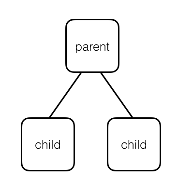
For the purpose of capsule networks, we’re going to model this piece-by-piece focus as a tree. Trees are made of parent nodes and descendant, children nodes. They are called trees because they are modeled after the shape of tree branches.

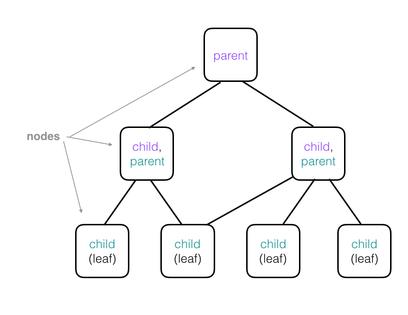
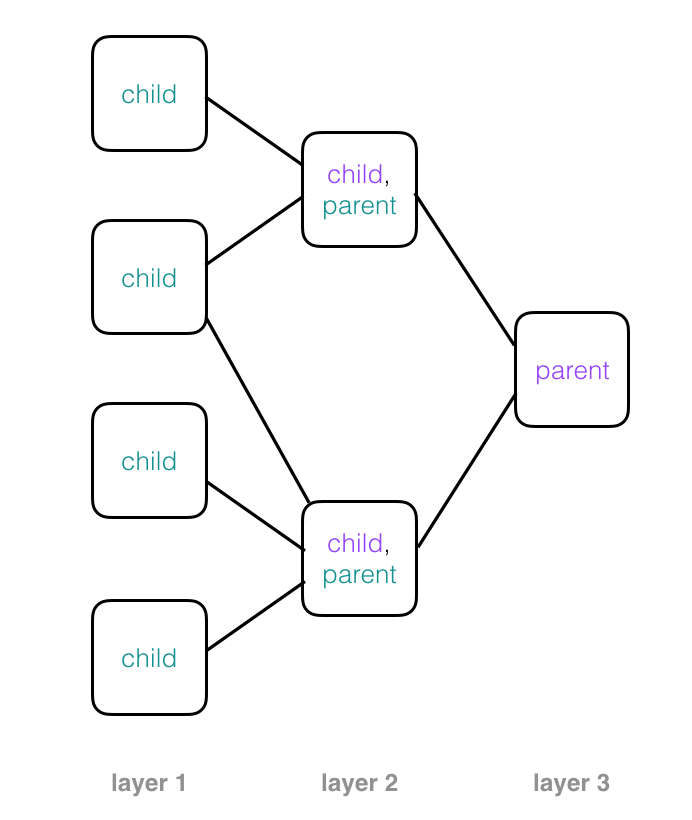
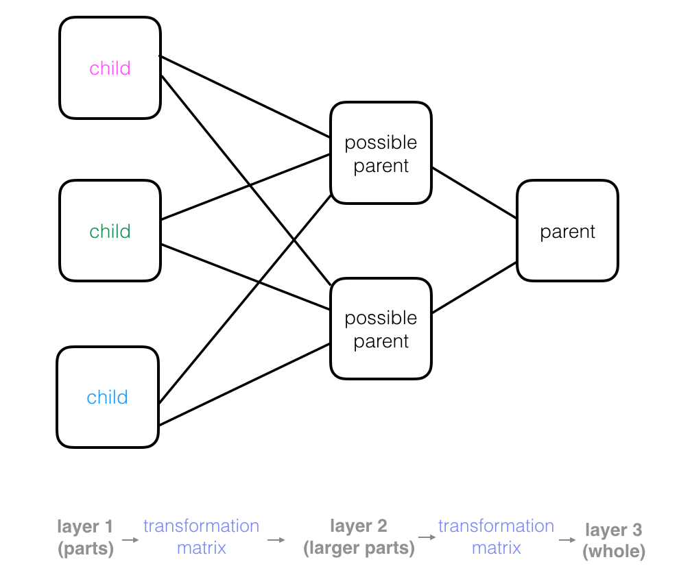
A more complex tree is pictured below. Note that the child nodes in higher layers are parents of their own child nodes; these have been color-coded in the diagram so that if a node is a child and parent, its child node text color matches it’s corresponding parent node’s text color. For example, a node that has purple “parent” text will be attached to a corresponding child node with a purple “child” label. Parent nodes may have more than one child and child nodes can be attached to multiple parents. Also, a “leaf” is a kind of child node without any children. In the case of capsule networks:

• Each node in a tree represents a single capsule.
• Each leaf represents a single, focused observation.

In the example below, you can see how the parts of a face (eyes, nose, mouth, etc.) might be recognized in leaf nodes and then combined to form a more complete face part in parent nodes.

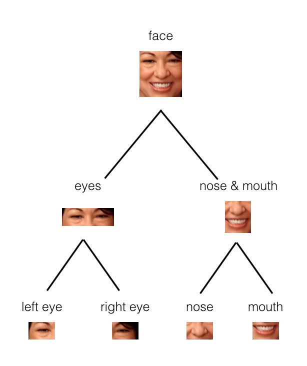
Parent nodes combine observations from child nodes to build up a more complex picture. In a neural network structure, you’ll often see these trees rotated so that they are on their side. This may start to look like a familiar image of a neural network, with layers of nodes that process some input data, produce outputs, and pass those outputs to the next layer of nodes.

Recall that every node in this tree represents a capsule in a capsule network, and as we move forward through these layers, the capsules in each layer can build up a more complete representation of an object in an image piece-by-piece. Next, let’s see how capsules represent image and object parts.

---

What is a Capsule?

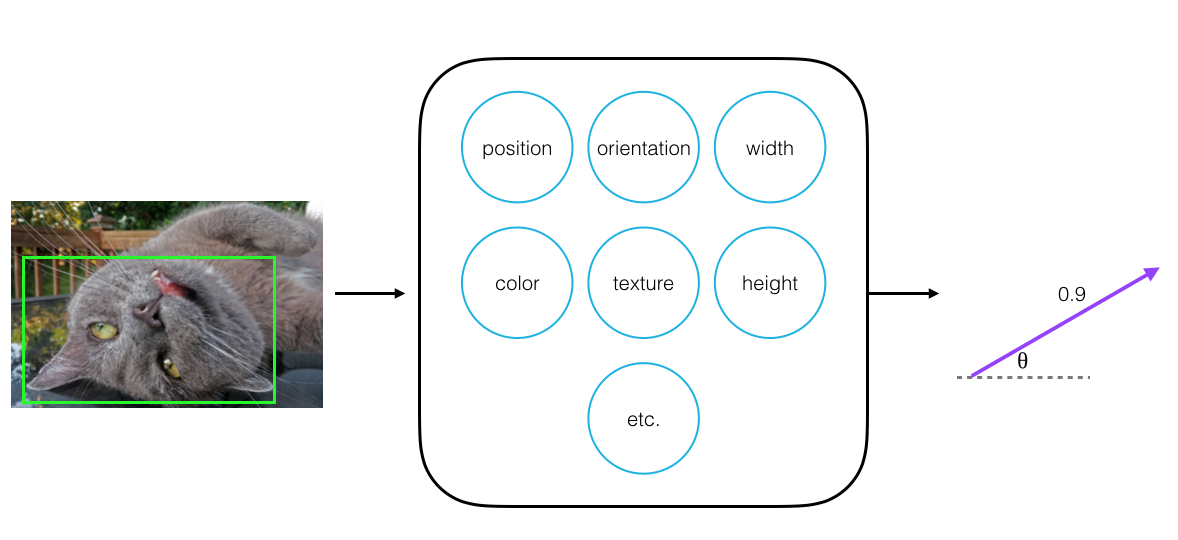
Capsules are a small group of neurons where each neuron in a capsule represents various properties of a particular image part. Some examples of part properties include: position and orientation in an image, width, and texture.

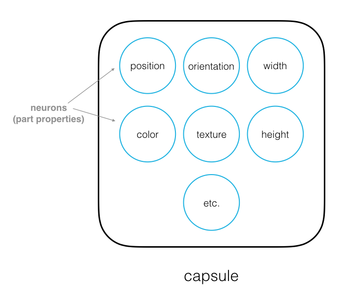
A special part property is its existence in an image.

Existence

We can represent a part’s existence in an image by a probability value: 0 if that part is not detected and 1 if it is; a value of 0.8 indicates an 80% confidence that the part has been found in the image. For example, say we are trying to identify a cat and one part we are trying to identify is a cat’s face. We could approach this task in a couple of ways. One way to find the existence of this part, in an image of a cat, is to perform a binary classification: contains-part or doesn’t-contain-part, and use those class scores to get the probability of existence. Another way is to look at all of the part properties in a capsule (the width and texture of the face, the angle the face is pointing, etc.) and say that the probability of existence is a function of the number of those properties. If a face-like shape is detected and a certain width and angle are identified, these property neurons will become active, and we can use this activity to indicate the existence of a part. This is the approach that capsules take, and it offers a number of advantages to the binary classification approach.

Output Vector

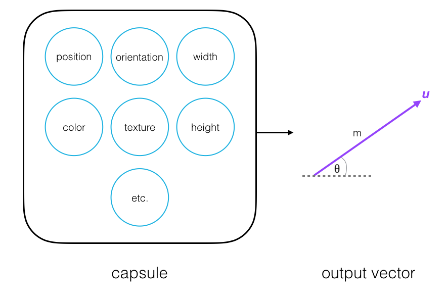
Every capsule outputs a vector, u, with a magnitude and orientation.

• Magnitude (m) = the probability that a part exists; a value between 0 and 1.
• Orientation (theta) = the state of the part properties.

• The magnitude of the vector is a value between 0 and 1 that indicates the probability that a part exists and has been detected in an image. This is a normalized function of the weighted inputs to a particular a capsule; a nonlinear function called squashing.

• The orientation of the vector represents the state of the part properties; this orientation will change if one of the part properties changes.

Going back to the cat face detection example, say a capsule detects a cat’s face in an image, and it outputs a vector with a magnitude of 0.9. This means that it detects a face with 90% confidence.

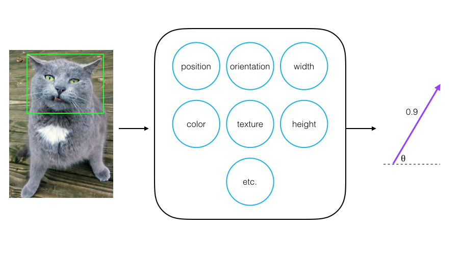
If we then look at a different image of this cat’s face, one in which the cat has flipped, the orientation of this capsule’s output vector will change. The face part properties, position, orientation, and shape, have changed in this new image, and the orientation of the output vector changes with each of these property changes. These changes are changes in neural activities inside a capsule. The magnitude of the vector should remain very close to 0.9 since the capsule should still be confident that the face exists in the image!

The Importance of a Vector

So, why have a vector output instead of a single value? Why is orientation a useful value?

The fact that the output of a capsule is a vector, with some orientation, makes it possible to use a powerful dynamic routing mechanism to ensure that the output of a capsule gets sent to the appropriate parent capsule in the next layer of capsules.

---

Dynamic Routing

Dynamic routing is a process for finding the best connections between the output of one capsule and the inputs of the next layer of capsules. It allows capsules to communicate with each other and determine how data moves through them, according to real-time changes in the network inputs and outputs! So, no matter what kind of input image a capsule network sees, dynamic routing ensures that the output of one capsule gets sent to the appropriate parent capsule in the following layer.

Routing Example: Maxpooling

You may have already seen an example of a simple routing process in a convolutional neural network. CNN’s extract features from images via a convolutional layer that is made of a stack of filtered images. In a typical CNN architecture, this filtered information is then passed to a maxpooling layer. (If you’d like to review this architecture, it’s covered in a previous post.) The maxpooling layer creates a route that ignores all but the most “active” or high-valued features in a patch in the previous, convolutional layer.

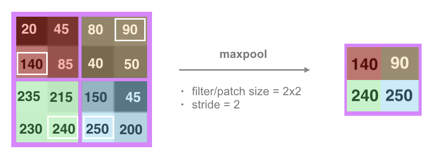
This routing process discards a lot of pixel information and it produces vastly different results for image of the same object in different orientations. So, how does dynamic routing work and how does it improve upon a simple routing process like maxpooling?

Coupling Coefficients

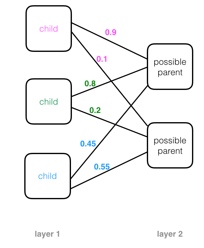
When a capsule network is initialized, child capsules are not sure where their outputs should go as they act as input to the next layer of parent capsules. In fact, each capsule starts out with a list of possible parents, which is all the parent capsules in the next layer. This possibility is represented by a value called the coupling coefficient, c, which is the probability that a certain capsule’s output should go to a parent capsule in the next layer. Examples of coupling coefficients, written on the connecting lines between a child and its possible parent nodes, are pictured below. A child node with two possible parents will start out with equal coupling coefficients for both: 0.5.

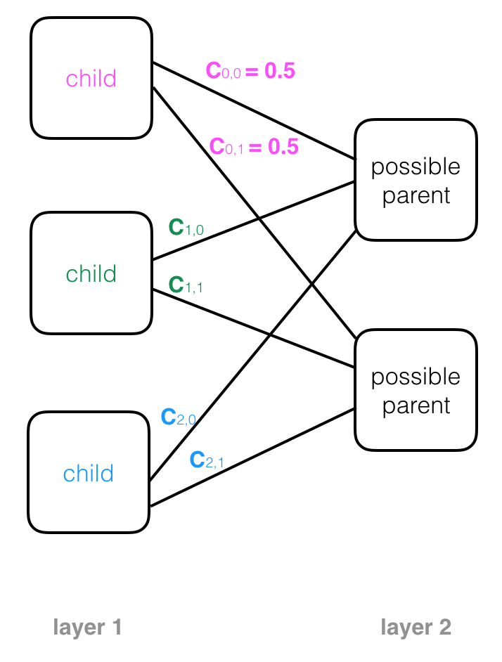
The coupling coefficients across all possible parents can be pictured as a discrete probability distribution. Across all connections between one child capsule and all possible parent capsules, the coupling coefficients should sum to 1.

Routing by Agreement

Dynamic routing is an iterative process that updates these coupling coefficients. The update process, performed during network training, is as follows for a single capsule:

• A child capsule represents a part of a whole object. Each child capsule produces some output vector u; its magnitude represents a part’s existence and its orientation represents the generalized pose of the part.

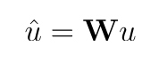
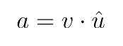
• For each possible parent, a child capsule computes a prediction vector, u_hat (^), which is a function of its output vector, u, times a weight matrix, W. You can think of W as a linear transformation—a translation or rotation, for example—that relates the pose of a part to the pose of a larger part or whole object (ex. if a nose is pointing to the left, the whole face it is a part of is likely also pointing left). Then u_hat (^) is a prediction about the pose of a larger part, represented by a parent capsule.

• If the prediction vector has a large dot product with the parent capsule output vector, v, then these vectors are said to agree and the coupling coefficient between that parent and the child capsule increases. Simultaneously, the coupling coefficient between that child capsule and all other parents decreases.

• This dot product between the parent output vector, v, and a prediction vector, u_hat, is known as a measure of capsule agreement, a.

This is sometimes referred to as top-down feedback; feedback from a later layer of parent capsule outputs.

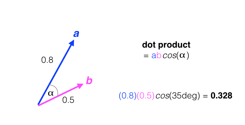
The dot product between two vectors is a single value that can be thought of as a measure of orientation similarity or alignment. Consider the two vectors, a and b, below. The dot product between a and b is calculated as their magnitudes times the cosine of the angle, alpha, between them: a*b*cos(alpha). Cosine is at a maximum value (1) if the two vectors have no angle difference between them, and is at a minimum (0) when the two vectors have a right-angle difference between them. In the example below, the dot product is calculated for two vectors with alpha equal to 35 degrees.

A high coupling coefficient, between a child and parent capsule, increases the contribution of the child to that parent, thus further aligning their two output vectors and making their agreement dot product even larger!

This is called routing by agreement. If the orientation of the output vectors of capsules in successive layers are aligned, then they agree that they should be coupled, and the connections between them are strengthened. The coupling coefficients are calculated by a softmax function that operates on the agreements, a, between capsules and turns them into probabilities such that the coefficients between one child, and its possible parents, sum to 1.

A typical training process may include three such agreement iterations and final coupling coefficients may look like the following image, with some child capsules choosing one dominant parent and others contributing to both parents.

Strengths & Attention

Dynamic routing can be viewed as a parallel attention mechanism that allows capsules at one level to “attend” to certain, active capsules in a previous layer and ignore others. It turns out that this routing mechanism is extremely good at identifying multiple objects even when they overlap.

---

Learning Spatial Relationships

During the training process, while figuring out appropriate coupling coefficients between child and parent capsules, a capsule network learns the spatial relationships between parts and their wholes.

For example, to recognize a face, a capsule network would need to know that a typical face has a left and right eye, and a nose and mouth below those eyes. Then, only if it sees those parts in their expected locations and orientations, relative to one another, a capsule network could put those parts together to identify a complete face.

The spatial relationships between parts can be modeled by a series of matrix multiplications, between the output of child capsules and parents, that capture the pose (the position and orientation) of each part; then a capsule network essentially checks for agreement between these poses. Agreement is based on the vector orientations of child and parent capsules, and when compared to the scalar outputs of a typical convolutional layer, a capsule’s vector output can provide more information.

For example, agreement can ensure that all the parts of a single face are facing in the same direction or that there are one or two eyes on a face and not three. This is in contrast to a typical CNN which only checks for the existence of different features, but not their relationship to one another.

Capsules use neural activities that vary with object orientation. They learn to represent spatial relationships between parts and whole objects, which makes it easier for a capsule network to identify an object no matter what orientation it is in.

---

Capsule Network Architecture & Implementation

A Capsule Network can be broken down into two main parts:

1. A convolutional encoder
2. A fully-connected, linear decoder

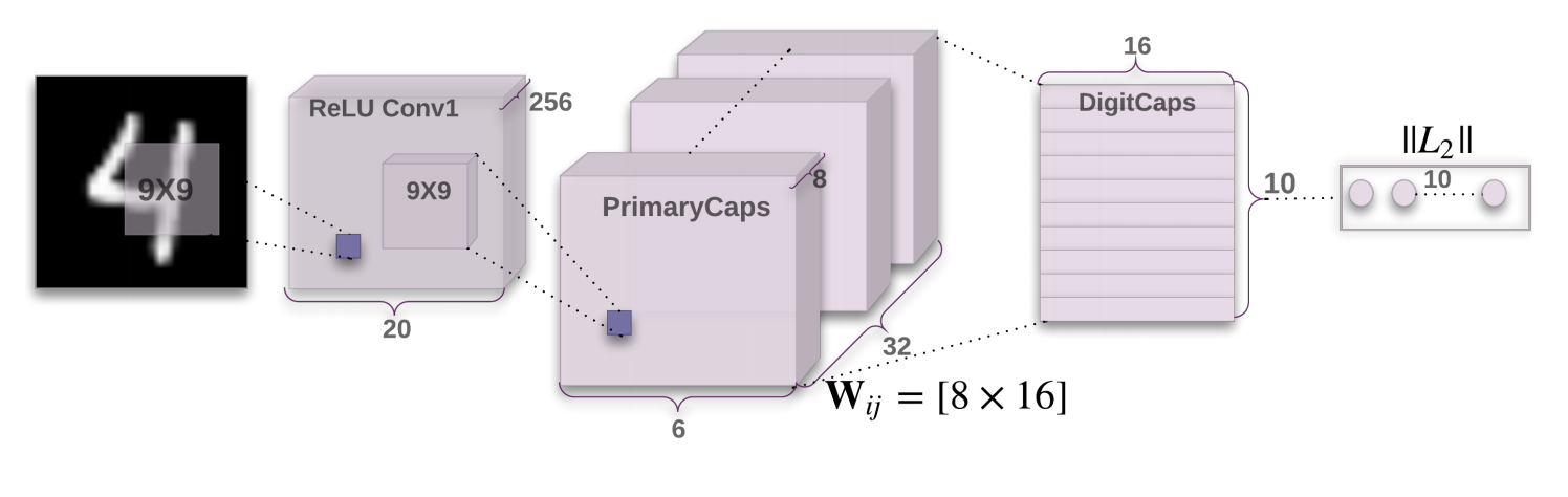
The above image was taken from the original Capsule Network paper (Hinton et. al.).

I’ve implemented the capsule network in PyTorch code and you can find that readable implementation in my Github repository. In the notebook, I define and train a simple Capsule Network that aims to classify MNIST images. The notebook follows the architecture described in the original paper and tries to replicate some of the experiments, such as feature visualization, that the authors pursued. I’ve taken note of some model attributes that I found particularly interesting, below, and I encourage you to read through the implementation or try to run the code, locally!

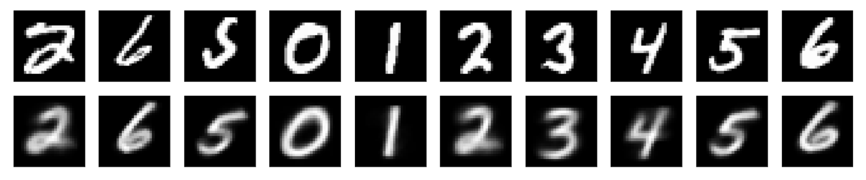
Decoder Reconstructions

The decoder sees as input the 16-dimensional vectors that are produced by the DigitCaps layer. There is one “correct” capsule output vector; this vector is the vector with the largest vector magnitude of all ten digit capsule outputs (recall that vector magnitude corresponds to a part’s existence in an image). Then, the decoder upsamples that one vector, decoding it into a reconstructed image of a handwritten digit. So, the decoder is learning a mapping from a capsule output vector to a 784-dim vector that can be reshaped into a 28x28 reconstructed image. You can see some sample reconstructions, below. The original images are on the top row, and their reconstructions are in the row below; you can see that the reconstructions are blurrier but, generally, quite good.

This will be a great visualization tool and this decoder acts as a regularization technique, forcing the 16-dimensional vectors to encode something about the content of an input image.

Output Vector Dimensions

The final capsule layer, DigitCaps, outputs vectors of length 16. It turns out that some of these vector dimensions have learned to represent the features that makeup and distinguish each class of handwritten digit, 0-9. The features that distinguish different image classes are traits like image width, skew, line thickness, and so on. In my implementation, I tried to visualize what each vector dimension represents by slightly modifying the capsule output vectors and visualizing the reconstructed images. I’ve highlighted some of my results below.

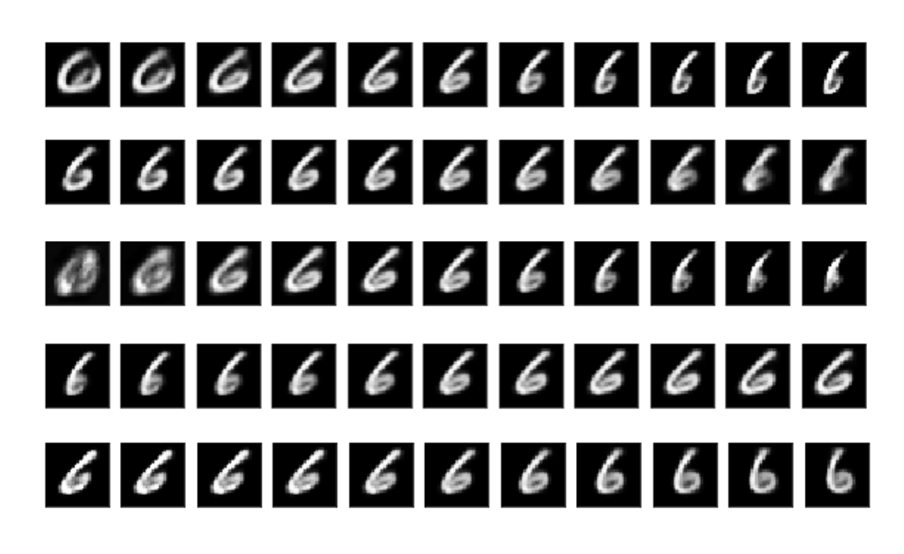
You can see all of these experiments and results in my complete implementation.

---

This post was edited on November 17, 2018.

If you are interested in my work and thoughts, check out my Twitter or connect with me on LinkedIn.